---
title: 'The Cost of a Minute: How Delivery Delays Define Customer Value'
subtitle: 'Customer Segmentation Analysis on Blinkit Sales dataset'
author:
- name: Utkarsh Tripathi
affiliation: BITS Pilani
- name: Juwaria Qadri
affiliation: BITS Pilani
- name: Mohammed Omar
affiliation: BITS Pilani
- name: Merin Ann Cherian
affiliation: BITS Pilani
date: 'today'
format:
html:
code-fold: true
toc: true
jupyter: python3
---
# 1. Project Overview
The notebook is divided into the following components:
- **Data Loading**: Importing the dataset.
- **Data Validation**: Initial checks for structure and quality.
- **Data Cleaning**: Preprocessing and handling missing values.
- **EDA**: Exploratory Data Analysis to uncover patterns.
- **Feature Engineering**: Creating new features for modelling.
- **Cluster Modelling**: Applying K-Means clustering.
- **Basic Inferences**: Deriving insights from the clusters.
```{python}
# Library imports
# Data Analytics
import pandas as pd
import numpy as np
# Data Viz
import seaborn as sns
import matplotlib.pyplot as plt
# scikit-learn
from sklearn.preprocessing import StandardScaler, RobustScaler, MinMaxScaler, OneHotEncoder
from sklearn.cluster import KMeans
from sklearn.decomposition import PCA
from sklearn.metrics import silhouette_score, davies_bouldin_score, calinski_harabasz_score
```
# 2. Data Loading
Loading a CSV dataset into the Pandas DataFrame.
```{python}
#| code-fold: false
# Dataset loading

input_path = "./blinkit_orders.csv"
df=pd.read_csv(input_path)
```
# 3. Data Validation
### Basic Data Exploration & Summary
The following functions are used to inspect the dataset structure and summary statistics:
- `basic_exploration(df)`: Prints shape, top rows, info, null counts, unique values, and duplicates.
- `summarize_df(df)`: Provides descriptive statistics and checks for anomalies (e.g., negative order totals).
```{python}
#| code-summary: "Click to see Data Validation Functions"
def basic_exploration(df):
    print("Shape of DataFrame:")
    print(df.shape)

    # Display top 5 rows
    print("Top 5 Rows:")
    display(df.head())

    # Basic info about the data
    print("Basic Information:")
    print(df.info())

    # Count null values and describe statistics
    print("Count of Null Values:")
    print(df.isnull().sum())

    print("Unique Value Counts per Column:", df.nunique(), sep="\n")

    print("Number of Duplicated Rows:", df.duplicated().sum())

def summarize_df(df):
    # Checking for anomalies
    display(df.describe(include='all'))

    # Categorical column summary
    display(df.describe(include=['object']))

    if 'order_total' in df.columns:
        invalid_order_total = df[df['order_total'] <= 0]
        print("Rows with Invalid (≤0) Order Total:")
        display(invalid_order_total)

basic_exploration(df)
summarize_df(df)
```
# 4. Data Cleaning
The data cleaning process involves several key steps to ensure data quality:
1. **Drop Irrelevant Columns**: Removing columns that do not contribute to analysis.
2. **Remove High Missing Value Columns**: Dropping features with >50% missing data.
3. **Impute Missing Values**:
- Numerical: Median
- Categorical: Mode
- Others: Forward Fill
4. **Remove Duplicates**: Eliminating identical rows.
5. **Handle Outliers**: Capping `order_total` using IQR (Interquartile Range).
6. **Date Conversions**: Parsing date columns to datetime objects.
7. **Feature Creation**: Calculating `delivery_delay_minutes`.
8. **Type Conversion**: Converting object columns to categorical types for efficiency.
```{python}
#| code-summary: "Click to see Data Cleaning Functions"
def drop_irrelevant_columns(df, irrelevant_cols):
    """Drop columns with irrelevant information."""
    for col in irrelevant_cols:
        if col in df.columns:
            df.drop(columns=[col], inplace=True)

def drop_high_missing_value_columns(df, threshold=0.5):
    """Remove columns with missing values above a certain threshold."""
    cols_to_drop = [col for col in df.columns if df[col].isnull().mean() >= threshold]
    df.drop(columns=cols_to_drop, inplace=True)

def impute_missing_values(df):
    """Impute missing values based on the data type of each column."""
    for col in df.columns:
        if df[col].dtype in ['float64', 'int64']:
            df[col] = df[col].fillna(df[col].median())
        elif df[col].dtype == 'object':
            df[col] = df[col].fillna(df[col].mode()[0])
        else:
            df[col] = df[col].ffill()

def remove_duplicates(df):
    """Remove duplicate rows."""
    before = df.shape[0]
    df.drop_duplicates(inplace=True)
    print(f"Removed {before - df.shape[0]} duplicate rows")

def handle_outliers(df, column='order_total'):
    """Handle outliers using IQR capping."""
    Q1 = df[column].quantile(0.25)
    Q3 = df[column].quantile(0.75)
    IQR = Q3 - Q1
    lower_bound = Q1 - 1.5 * IQR
    upper_bound = Q3 + 1.5 * IQR

    df.loc[df[column] < lower_bound, column] = lower_bound
    df.loc[df[column] > upper_bound, column] = upper_bound

def convert_to_datetime(df, columns):
    """Convert date/time columns to datetime."""
    for col in columns:
        if col in df.columns:
            df[col] = pd.to_datetime(df[col], dayfirst=False, errors='coerce')

def calculate_delivery_delay(df):
    """Calculate delivery delay (in minutes)."""
    df['delivery_delay_minutes'] = (df['actual_delivery_time'] -
                                    df['promised_delivery_time']).dt.total_seconds() / 60

def convert_categorical_like_columns(df, columns):
    """Convert categorical-like columns to category type."""
    for col in columns:
        if col in df.columns:
            df[col] = df[col].astype('category')

def save_cleaned_dataset(df):
    """Save the cleaned dataset to a CSV file."""
    # df.to_csv(filename, index=False)
    print("Data cleaning completed successfully!")
    print("Final Data Shape:", df.shape)
    print("Data Types:", df.dtypes, sep='\n')
    return df
```
### Execution of Data Cleaning
We apply the defined cleaning pipeline to our dataframe.
```{python}
# List of irrelevant columns (example placeholder)
irrelevant_cols = ['irrelevant_column']

# Columns with high missing values threshold
threshold_high_missing_values = 0.5

# Categorical-like columns to convert
categorical_like_columns = ['payment_method', 'delivery_status']

drop_irrelevant_columns(df, irrelevant_cols)
drop_high_missing_value_columns(df, threshold=threshold_high_missing_values)
impute_missing_values(df)
remove_duplicates(df)
handle_outliers(df)
convert_to_datetime(df, columns=['order_date','actual_delivery_time', 'promised_delivery_time'])
calculate_delivery_delay(df)
convert_categorical_like_columns(df, categorical_like_columns)

# Save the cleaned dataset
df_cleaned = save_cleaned_dataset(df)
```
# 5. Exploratory Data Analysis (EDA)
We explore the dataset to understand key distributions, relationships, and customer behaviors.
## Statistical Summary
We begin with a statistical overview of the dataset columns.
- **Numerical Columns**: Descriptive stats for order totals and delivery delays.
- **Correlation**: Checking the relationship between spending and delays.
- **Categorical Columns**: Analyzing distributions of payment methods and delivery status.
- **Store Performance**: Comparing delivery performance across stores.
- **Daily Trends**: Aggregating sales over time.
```{python}
#| code-summary: "Click to see EDA Helper Functions"
def print_numerical_columns(df):
    """Print numerical columns with descriptive stats."""
    print("Numerical Columns")
    print("Descriptive stats", df[['order_total', 'delivery_delay_minutes']].describe(), sep="\n")
    print("\nDistribution of Spending", df[['order_total']].quantile([0.25, 0.5, 0.75, 0.95]), sep="\n")

def print_correlation(df):
    """Print correlation between numerical columns."""
    print("Correlation between order total and delivery delay in minutes",
          df[['order_total', 'delivery_delay_minutes']].corr(), sep="\n")

def print_categorical_columns(df):
    """Print categorical columns with distribution overview."""
    print("\nCategorical Columns")
    print("Payment Methods Distribution", df['payment_method'].value_counts(), sep="\n")
    print("Delivery Status Distribution",
          (df['delivery_status'].value_counts(normalize=True) * 100).round(2), sep="\n")

def filter_significantly_delayed_orders(df):
    """Filter and print significantly delayed orders."""
    significantly_delayed_orders = df[df['delivery_status'] == 'Significantly Delayed']
    count_delayed = significantly_delayed_orders.shape[0]
    print("Significantly delayed orders:", sep='\n')
    display(significantly_delayed_orders.head(5))
    display(count_delayed)

def generate_customer_summary(df):
    """Generate a summary table for each customer."""
    customer_summary = df.groupby('customer_id').agg({
        'order_total': 'sum',
        'order_id': 'count',
        'delivery_delay_minutes': 'mean'
    }).rename(columns={
        'order_total': 'total_spent',
        'order_id': 'order_count',
        'delivery_delay_minutes': 'avg_delivery_delay'
    }).sort_values(by='order_count', ascending=False)
    print("Summary Table for Each Customer:", sep='\n')
    display(customer_summary.head(10))

def generate_payment_method_summary(df):
    """Generate a summary table for payment methods."""
    payment_summary_df = df.groupby('payment_method', observed=True).agg({
        'order_total': 'mean',
        'order_id': 'count'
    }).rename(columns={
        'order_total': 'avg_order_value',
        'order_id': 'num_orders'
    })
    print("Payment Method Summary:")
    display(payment_summary_df)

def store_wise_order_total_by_delivery_status(df):
    """Generate a pivot table for order total by delivery status per store."""
    pivot_table = pd.pivot_table(df,
                                 index='store_id',
                                 columns='delivery_status',
                                 values='order_total',
                                 aggfunc='sum',
                                 fill_value=0,
                                 observed=False)
    print("Store-Wise Order Total by Delivery Status:")
    display(pivot_table)

def daily_sales_patterns(df):
    """Generate daily sales patterns."""
    daily_sales_df = df.set_index('order_date').resample('D').agg({
        'order_total': 'sum',
        'order_id': 'count'
    }).rename(columns={
        'order_total': 'total_sales',
        'order_id': 'num_orders'
    }).sort_index(level=1, ascending=False)
    print("Daily Sales Patterns:")
    display(daily_sales_df.head(10))
```
```{python}
print_numerical_columns(df_cleaned)
print_correlation(df_cleaned)
print_categorical_columns(df_cleaned)
filter_significantly_delayed_orders(df_cleaned)
generate_customer_summary(df_cleaned)
generate_payment_method_summary(df_cleaned)
store_wise_order_total_by_delivery_status(df_cleaned)
daily_sales_patterns_df = daily_sales_patterns(df_cleaned)
```
## Visualisation
We perform detailed visualisation to validate our statistical findings.
- **Univariate Analysis**: Histograms and boxplots for individual features.
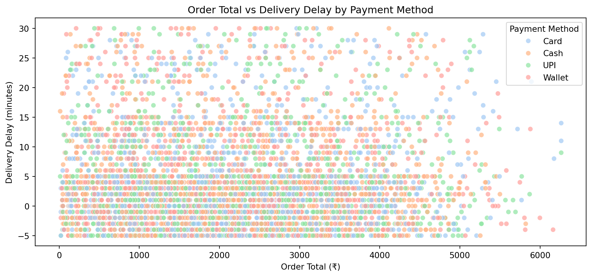
- **Bivariate & Multivariate**: Scatter plots to explore interaction effects (e.g., *Order Total vs Delivery Delay*).
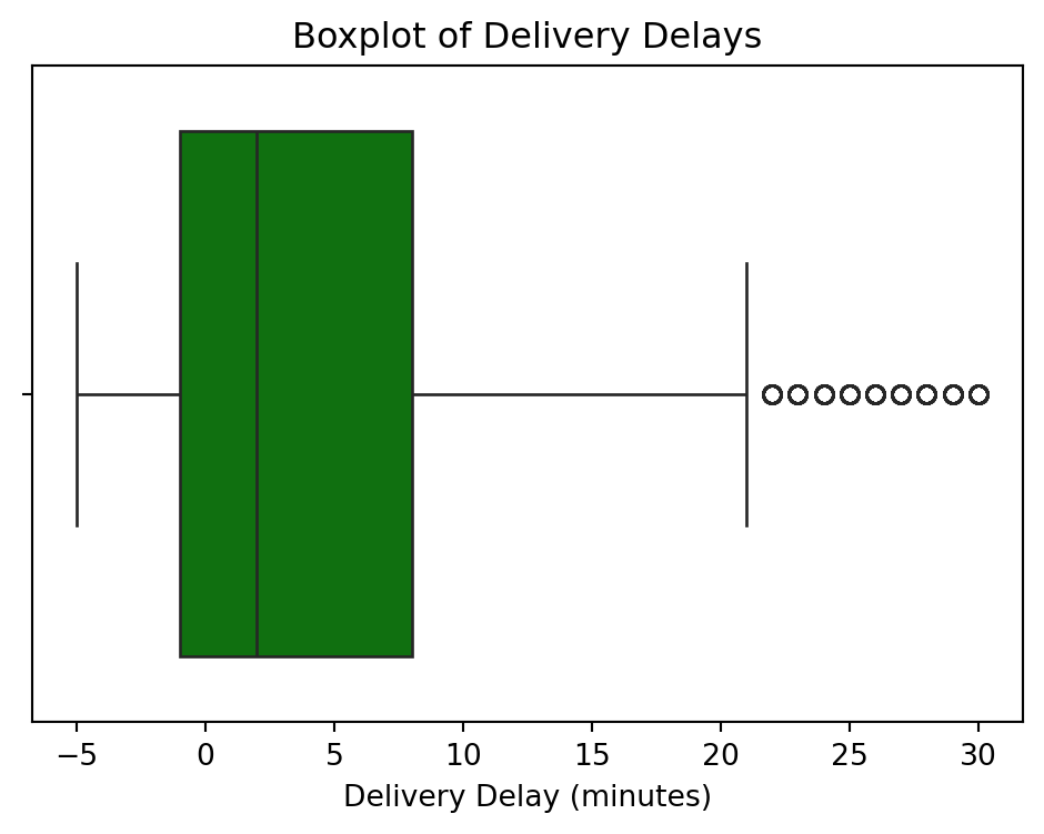
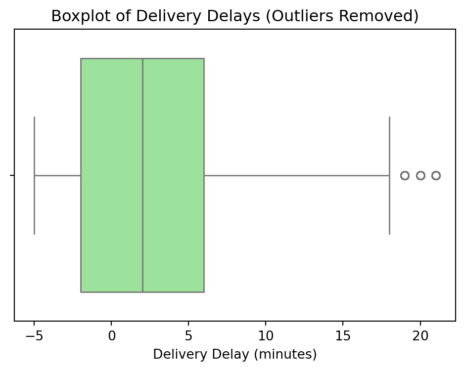
- **Outlier Detection**: Visualizing and removing extensive outliers in delivery delays.
```{python}
#| code-summary: "Click to see Visualization Functions"
def univariate_numeric_features(df):
"""Univariate analysis for numeric features."""
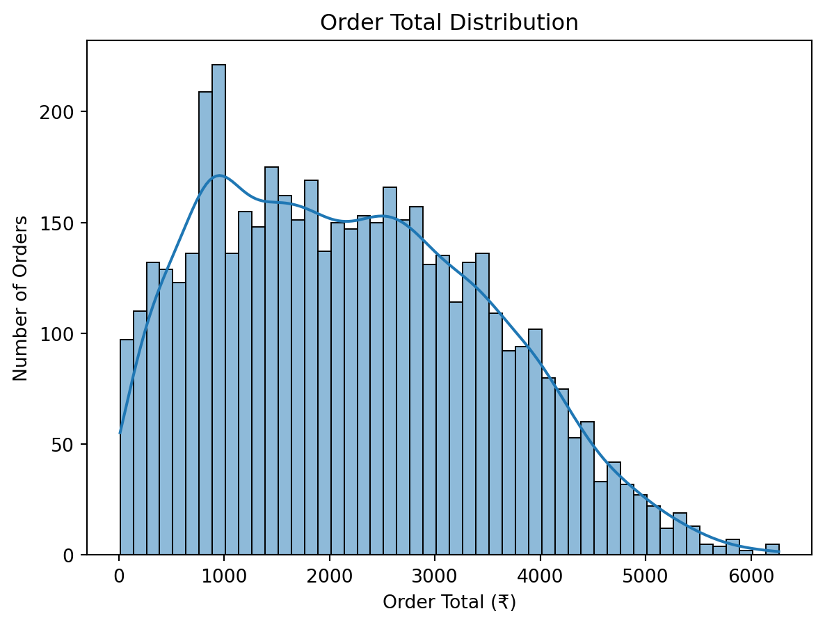
# Order Total Distribution
sns.histplot(df['order_total'], kde=True, bins=50)
plt.title('Order Total Distribution')
plt.xlabel('Order Total (₹)')
plt.ylabel('Number of Orders')
plt.show()
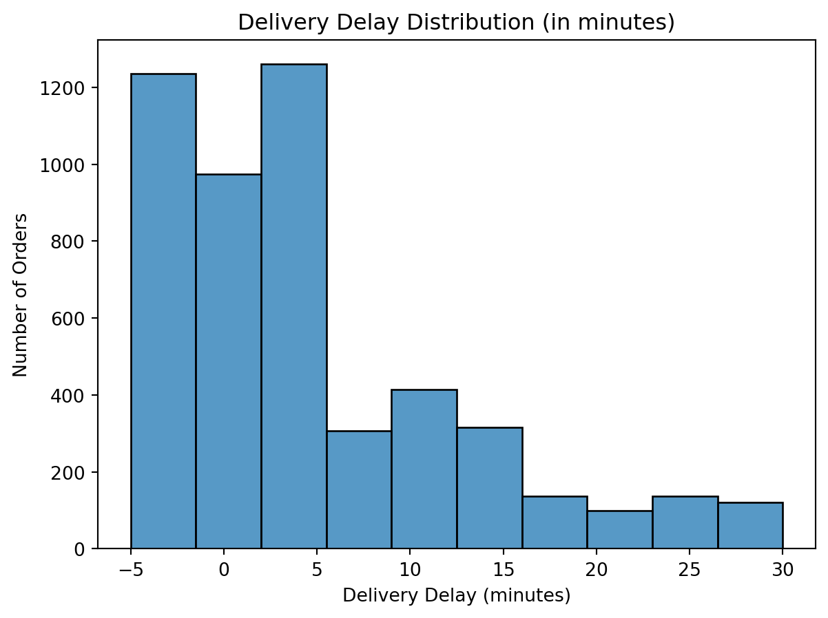
# Delivery Delay Distribution
sns.histplot(df['delivery_delay_minutes'], bins=10)
plt.title('Delivery Delay Distribution (in minutes)')
plt.xlabel('Delivery Delay (minutes)')
plt.ylabel('Number of Orders')
plt.show()
def univariate_categorical_features(df):
"""Univariate analysis for categorical features."""
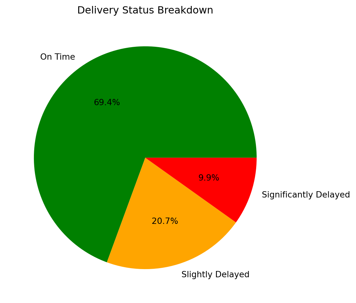
# Delivery Status Breakdown
delivery_counts = df['delivery_status'].value_counts()
plt.figure(figsize=(6, 6))
plt.pie(delivery_counts, labels=delivery_counts.index, autopct='%1.1f%%', colors=['green', 'orange', 'red'])
plt.title("Delivery Status Breakdown")
plt.show()
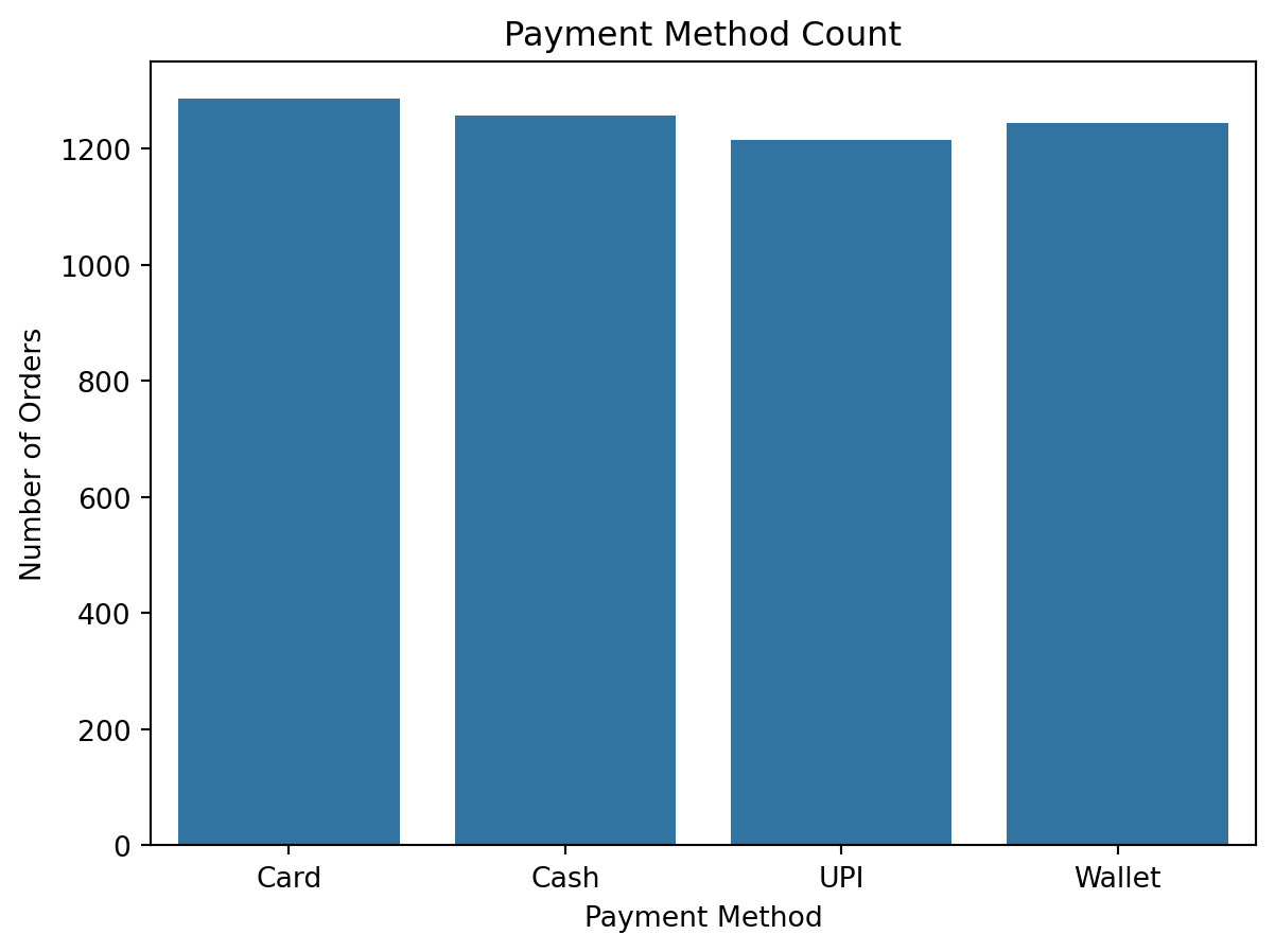
# Payment Method Count
sns.countplot(x='payment_method', data=df)
plt.title('Payment Method Count')
plt.xlabel('Payment Method')
plt.ylabel('Number of Orders')
plt.show()
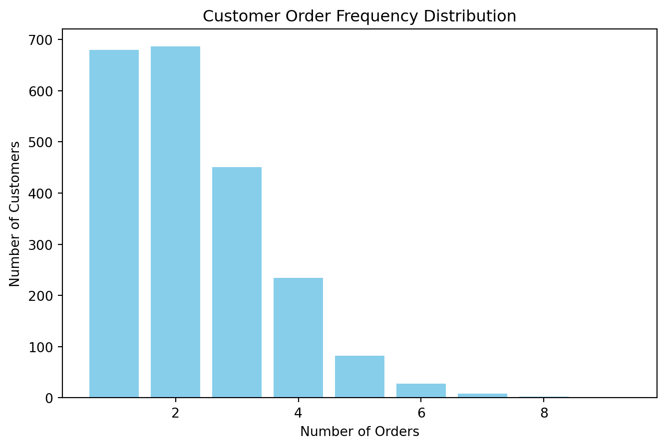
def univariate_customer_metrics(df):
"""Univariate analysis for customer metrics."""
# Customer Frequency Distribution
order_frequency_dist = df.groupby('customer_id').agg(
total_orders=('order_id', 'count'), # Total orders
total_spent=('order_total', 'sum'), # Lifetime value
avg_order_value=('order_total', 'mean') # Average order value
)['total_orders'].value_counts().sort_index()
print(order_frequency_dist)
plt.figure(figsize=(8, 5))
plt.bar(order_frequency_dist.index, order_frequency_dist.values, color='skyblue')
plt.xlabel("Number of Orders")
plt.ylabel("Number of Customers")
plt.title("Customer Order Frequency Distribution")
plt.show()
def univariate_one_time_vs_repeat_customers(df):
"""Univariate analysis for one-time vs repeat customers."""
customer_order_counts = df.groupby('customer_id').size()
print(f"One-time customers: {customer_order_counts[customer_order_counts == 1].count()}")
print(f"Repeat customers: {customer_order_counts[customer_order_counts > 1].count()}")
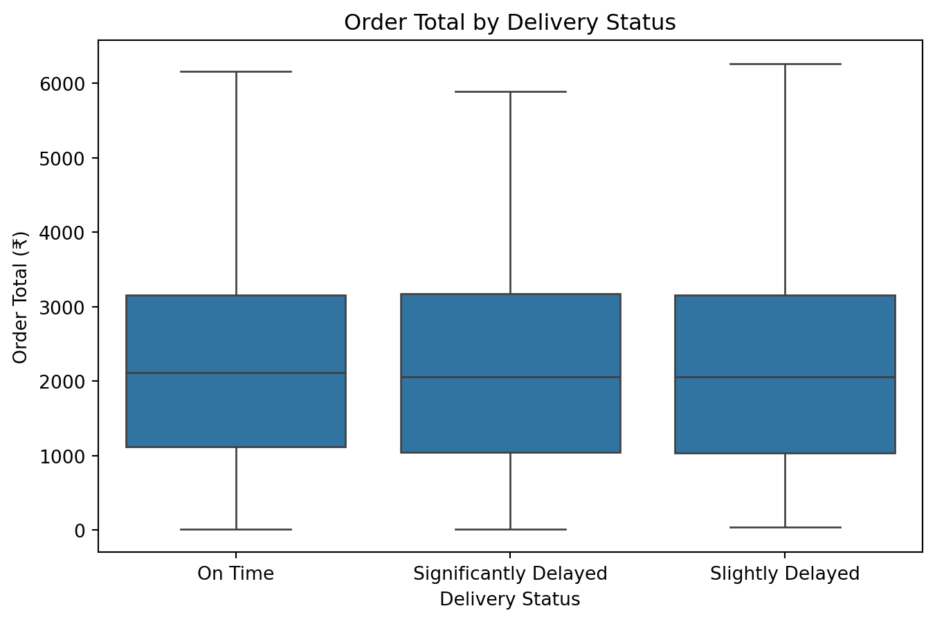
def bivariate_analysis(df):
"""Bivariate analysis."""
# Compare order amounts for On Time vs. Delayed deliveries
plt.figure(figsize=(8, 5))
sns.boxplot(x='delivery_status', y='order_total', data=df)
plt.title("Order Total by Delivery Status")
plt.xlabel("Delivery Status")
plt.ylabel("Order Total (₹)")
plt.show()
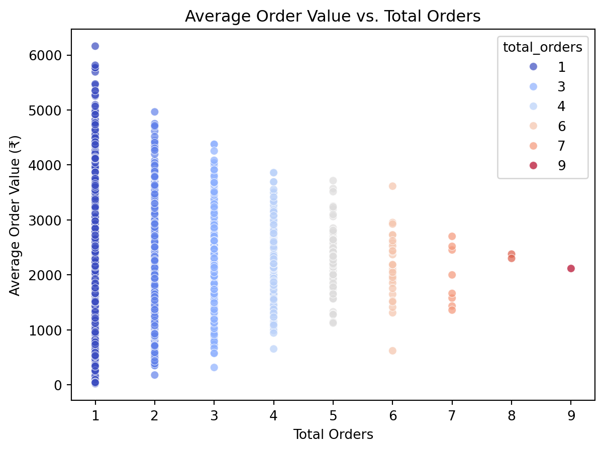
# Customer Spending Patterns
customer_metrics = df.groupby('customer_id').agg(
total_orders=('order_id', 'count'),
total_spent=('order_total', 'sum'),
avg_order_value=('order_total', 'mean')
)
sns.scatterplot(
data=customer_metrics,
x='total_orders',
y='avg_order_value',
hue='total_orders',
palette='coolwarm',
alpha=0.7
)
plt.title("Average Order Value vs. Total Orders")
plt.xlabel("Total Orders")
plt.ylabel("Average Order Value (₹)")
plt.show()
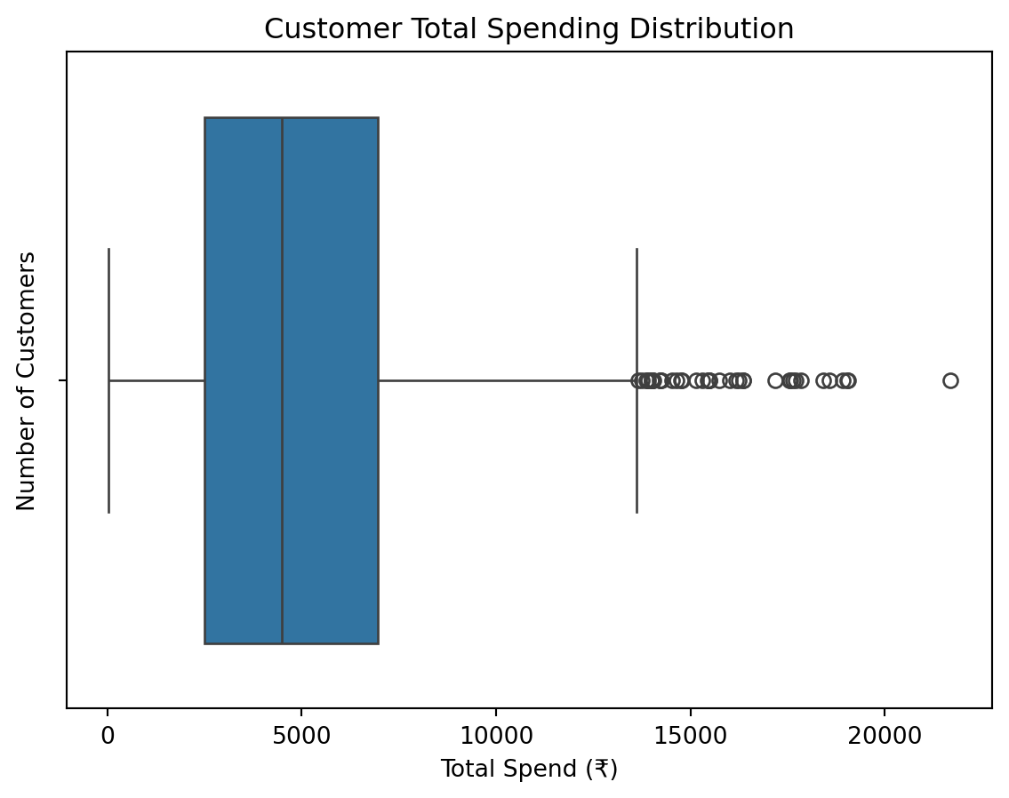
# Aggregate total spend per customer and visualize
customer_spending = df.groupby('customer_id')['order_total'].sum()
sns.boxplot(x=customer_spending)
plt.title("Customer Total Spending Distribution")
plt.xlabel("Total Spend (₹)")
plt.ylabel("Number of Customers")
plt.show()
plt.figure(figsize=(8, 5))
plt.hist(customer_spending, bins=20, color='skyblue', edgecolor='black')
plt.title("Customer Spending Distribution")
plt.xlabel("Total Spend (₹)")
plt.ylabel("Number of Customers")
plt.show()
def multivariate_analysis(df):
"""Multivariate analysis."""
# Relationship Between Order Total and Delivery Delay
plt.figure(figsize=(12, 5))
sns.scatterplot(
x='order_total',
y='delivery_delay_minutes',
hue='payment_method',
data=df,
alpha=0.7,
palette='pastel'
)
plt.title("Order Total vs Delivery Delay by Payment Method")
plt.xlabel("Order Total (₹)")
plt.ylabel("Delivery Delay (minutes)")
plt.legend(title="Payment Method")
plt.show()
def boxplot_delivery_delays(df):
"""Plot a boxplot of delivery delays."""
plt.figure(figsize=(6, 4))
sns.boxplot(x=df['delivery_delay_minutes'], color='green')
plt.title("Boxplot of Delivery Delays")
plt.xlabel("Delivery Delay (minutes)")
plt.show()
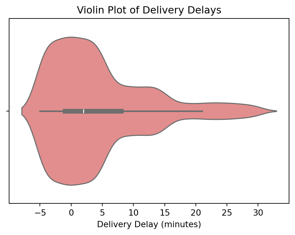
def violin_plot_delivery_delays(df):
"""Plot a violin plot of delivery delays."""
plt.figure(figsize=(6, 4))
sns.violinplot(x=df['delivery_delay_minutes'], color='lightcoral')
plt.title("Violin Plot of Delivery Delays")
plt.xlabel("Delivery Delay (minutes)")
plt.show()
def remove_outliers_delivery_delays(df):
"""Remove outliers from delivery delays and plot the boxplot."""
# Calculate Q1, Q3, and IQR
Q1 = df['delivery_delay_minutes'].quantile(0.25)
Q3 = df['delivery_delay_minutes'].quantile(0.75)
IQR = Q3 - Q1
# Filter out outliers
df_cleaned = df[(df['delivery_delay_minutes'] >= (Q1 - 1.5 * IQR)) &
(df['delivery_delay_minutes'] <= (Q3 + 1.5 * IQR))]
# Plot boxplot without outliers
plt.figure(figsize=(6, 4))
sns.boxplot(x=df_cleaned['delivery_delay_minutes'], color='lightgreen')
plt.title("Boxplot of Delivery Delays (Outliers Removed)")
plt.xlabel("Delivery Delay (minutes)")
plt.show()
return df_cleaned
```
```{python}
univariate_numeric_features(df_cleaned)
univariate_categorical_features(df_cleaned)
univariate_customer_metrics(df_cleaned)
univariate_one_time_vs_repeat_customers(df_cleaned)
bivariate_analysis(df_cleaned)
multivariate_analysis(df_cleaned)
boxplot_delivery_delays(df_cleaned)
violin_plot_delivery_delays(df_cleaned)
```
The delivery delay data shows significant outliers. We apply IQR filtering to clean this distribution.
```{python}
df_cleaned = remove_outliers_delivery_delays(df_cleaned)

# Save the cleaned dataset again after outlier removal
# df_cleaned = save_cleaned_dataset(df_cleaned, 'cleaned_data.csv')
```
### Final Data Inspection
```{python}
df_cleaned.head(5)
```
```{python}
df_cleaned['delivery_delay_minutes'].describe()
```
# 6. Feature Engineering
We transform raw transactional data into customer-centric features to prepare for clustering.
## Key Transformation Steps
1. **Aggregation**: Grouping by `customer_id` to calculate metrics:
- `avg_order_total`: Mean value of orders.
- `total_spent`: Sum of all orders.
- `num_orders`: Count of orders.
- `avg_delay`: Mean delivery delay.
- `most_used_payment`: Mode of payment method.
- `most_delivery_status`: Mode of delivery status.
2. **Encoding**: One-hot encoding categorical variables (`most_used_payment`, `most_delivery_status`).
3. **Scaling & Normalization**:
- **StandardScaler**: For `avg_order_total`.
- **Log Transform + StandardScaler**: For `total_spent` to handle skewness.
- **RobustScaler**: For `avg_delay` to handle outliers.
- **MinMax Scaler**: For `num_orders` to range (-1, 1).
```{python}
#| code-summary: "Click to see Feature Engineering Functions"
def aggregate_customer_data(df_cleaned):
# Aggregating customer data
customer_df = df_cleaned.groupby('customer_id').agg({
'order_total': ['mean', 'sum', 'count'],
'delivery_delay_minutes': 'mean',
'payment_method': lambda x: x.mode()[0],
'delivery_status': lambda x: x.mode()[0]
}).reset_index()
# Renaming columns
customer_df.columns = [
'customer_id', 'avg_order_total', 'total_spent', 'num_orders',
'avg_delay', 'most_used_payment', 'most_delivery_status'
]
return customer_df
def one_hot_encode_categorical_features(df):
# One-hot encoding categorical features separately
df_temp = df.copy()
one_hot = pd.get_dummies(df_temp[['most_used_payment', 'most_delivery_status']], prefix=['payment', 'status'])
df_final = pd.concat([df_temp.drop(columns=['most_used_payment', 'most_delivery_status']), one_hot], axis=1)
return df_final
def handle_numerical_features(df):
# Standardize avg_order_total
scaler = StandardScaler()
df['avg_order_total'] = scaler.fit_transform(df[['avg_order_total']])
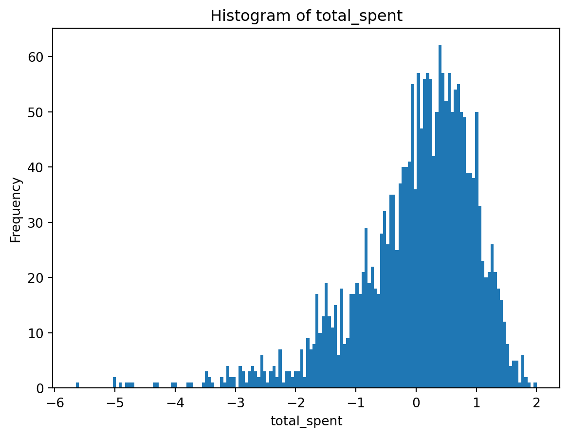
# Log transformation for total_spent to fix skewness
df['total_spent'] = np.log1p(df['total_spent'])
scaler = StandardScaler()
df['total_spent'] = scaler.fit_transform(df[['total_spent']])
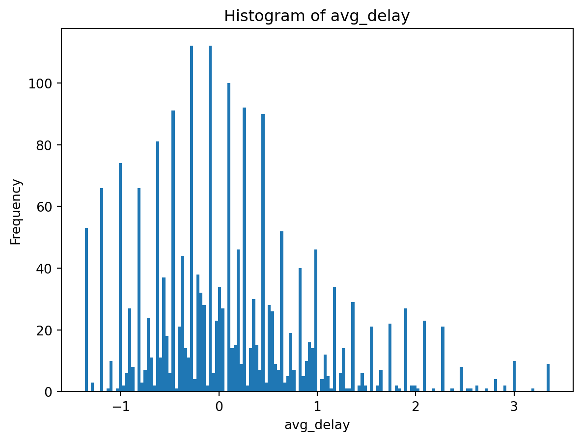
# Robust scaling for avg_delay
scaler = RobustScaler()
df['avg_delay'] = scaler.fit_transform(df[['avg_delay']])
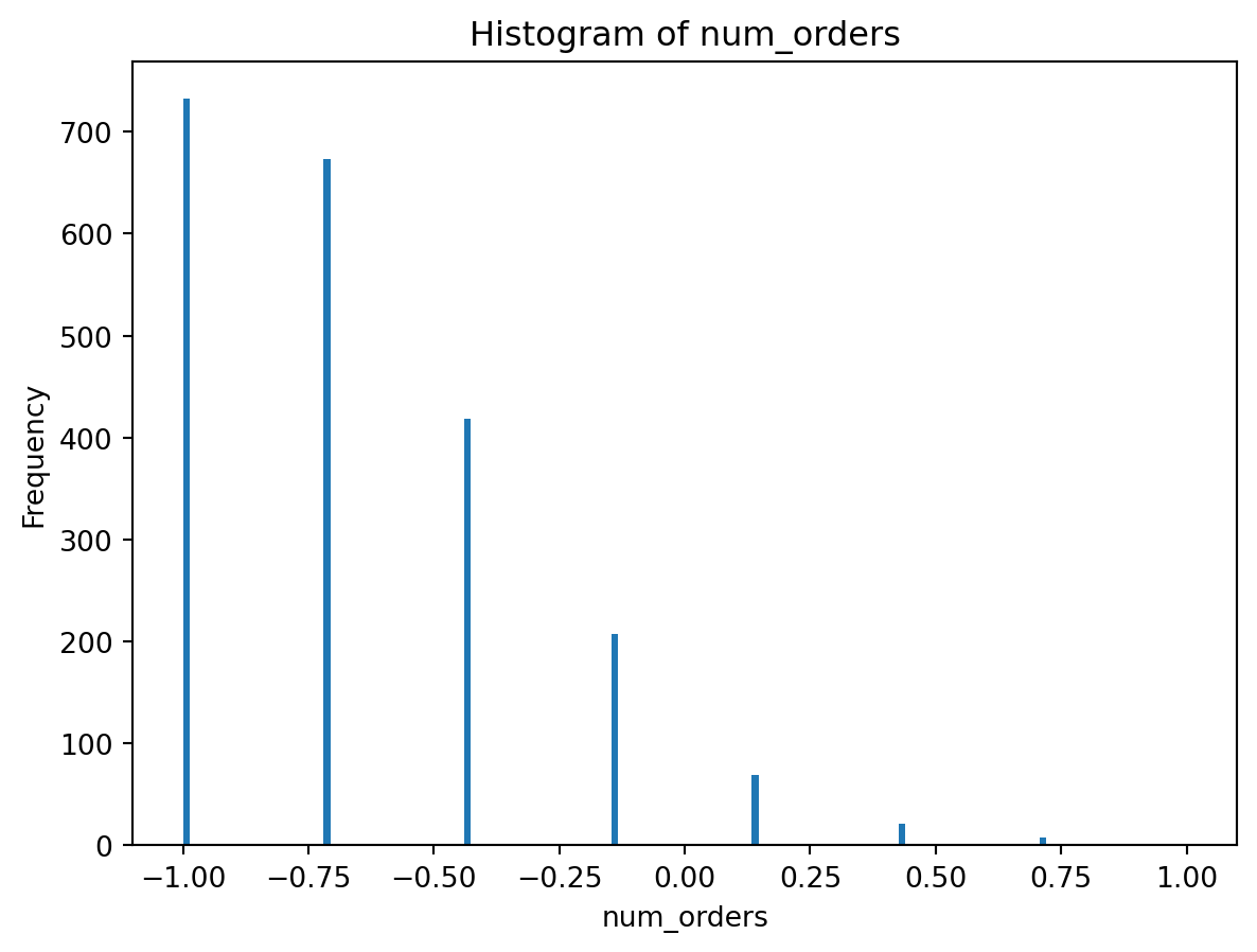
# MinMax scaling for num_orders
scaler = MinMaxScaler(feature_range=(-1, 1))
df['num_orders'] = scaler.fit_transform(df[['num_orders']])
return df
def process_customer_data(df_cleaned):
customer_df = aggregate_customer_data(df_cleaned)
customer_df_original=customer_df
one_hot_encoded_df = one_hot_encode_categorical_features(customer_df)
processed_df = handle_numerical_features(one_hot_encoded_df)
# Visualizations
plot_correlation_matrix(processed_df)
plot_histogram(processed_df['avg_order_total'])
plot_histogram(processed_df['total_spent'])
plot_histogram(processed_df['avg_delay'])
plot_histogram(processed_df['num_orders'])
return processed_df,customer_df_original
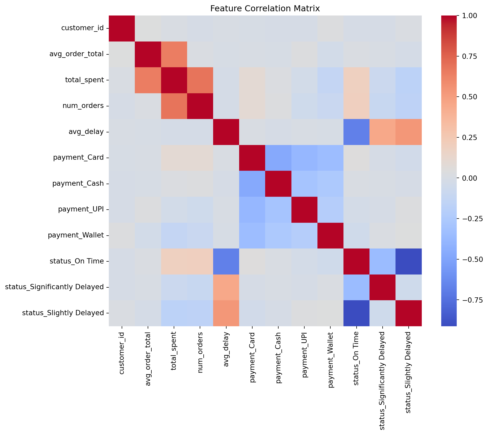
def plot_correlation_matrix(df):
plt.figure(figsize=(10, 8))
sns.heatmap(df.corr(), cmap='coolwarm', annot=False)
plt.title("Feature Correlation Matrix")
plt.show()
def plot_histogram(feature):
plt.hist(feature, bins=150)
plt.xlabel(feature.name)
plt.ylabel('Frequency')
plt.title(f'Histogram of {feature.name}')
plt.show()
```
### Execution
We process the data and visualize the distribution of updated features.
```{python}
customer_df, customer_df_original = process_customer_data(df_cleaned)

# Final Scaling adjustments (redundant but included for consistency with original script)
scaler = RobustScaler()
customer_df['avg_delay'] = scaler.fit_transform(customer_df[['avg_delay']])

scaler = MinMaxScaler(feature_range=(-1, 1))
customer_df['num_orders'] = scaler.fit_transform(customer_df[['num_orders']] )
customer_df[customer_df.select_dtypes('bool').columns] = customer_df.select_dtypes('bool').astype(int)
```
## Dataset Finalization
We remove identifiers and perform a final standard scaling on the entire dataset to ensure uniformity for the clustering algorithm.
```{python}
customer_df = customer_df.drop(['customer_id'], axis=1)
scaler = StandardScaler()
X_scaled = scaler.fit_transform(customer_df)

# Save processed data
# customer_df.to_csv('customer_df_processed.csv')

# Preview
customer_df.head(5)
```
# 7. Cluster Modelling
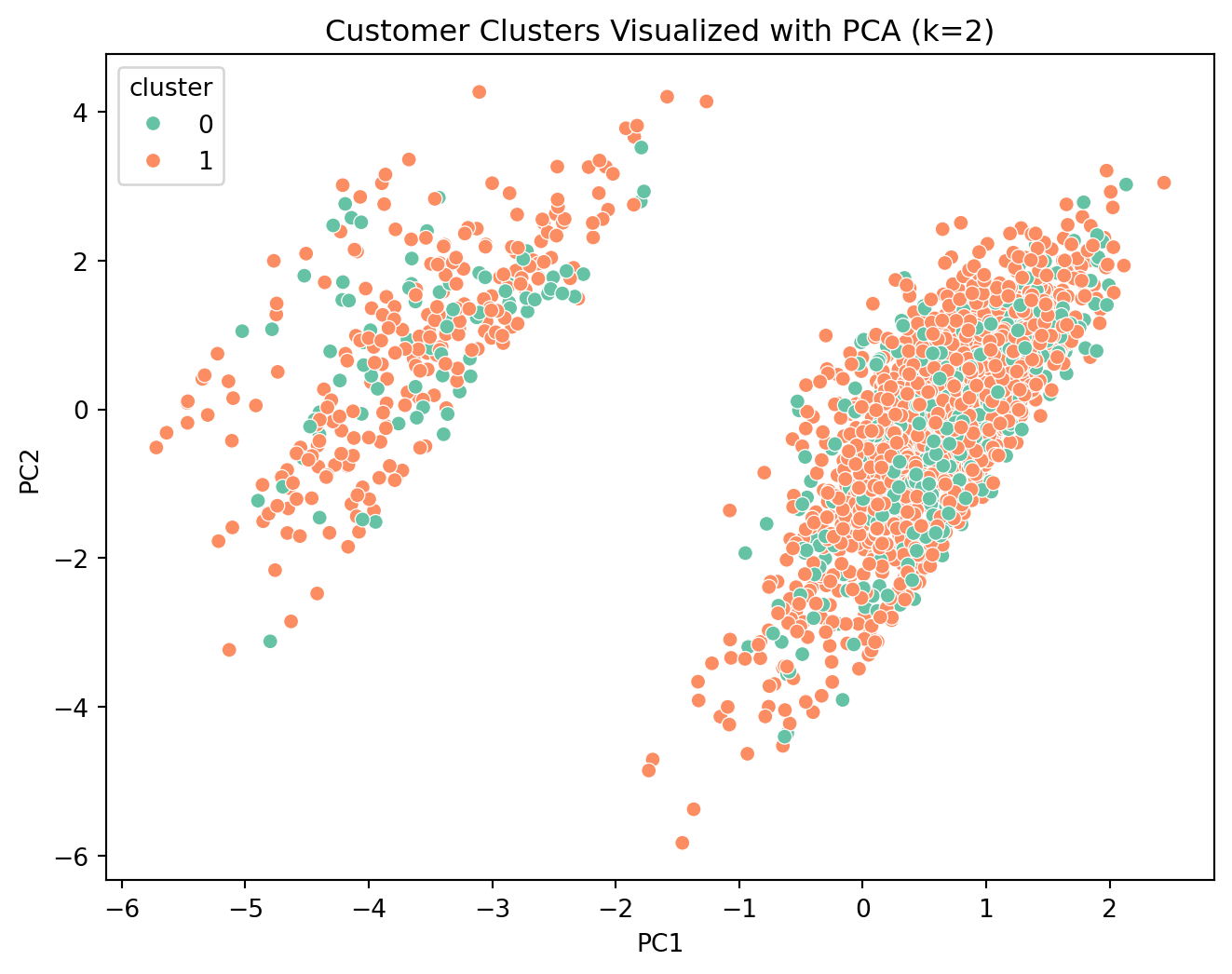
We employ **K-Means Clustering** to segment customers. To determine the optimal number of segments (*k*), we evaluate multiple scenarios using key performance metrics.
## Methodology
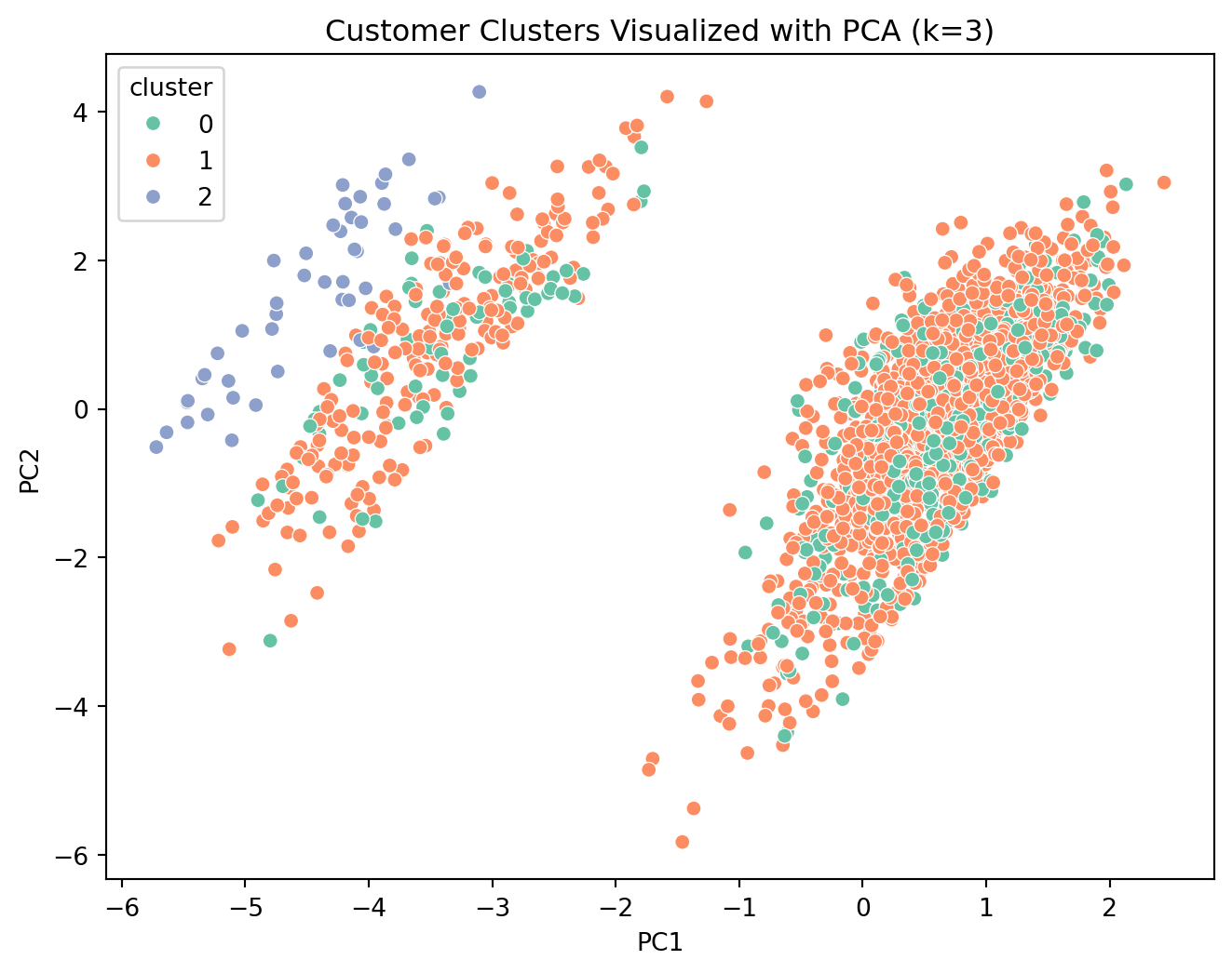
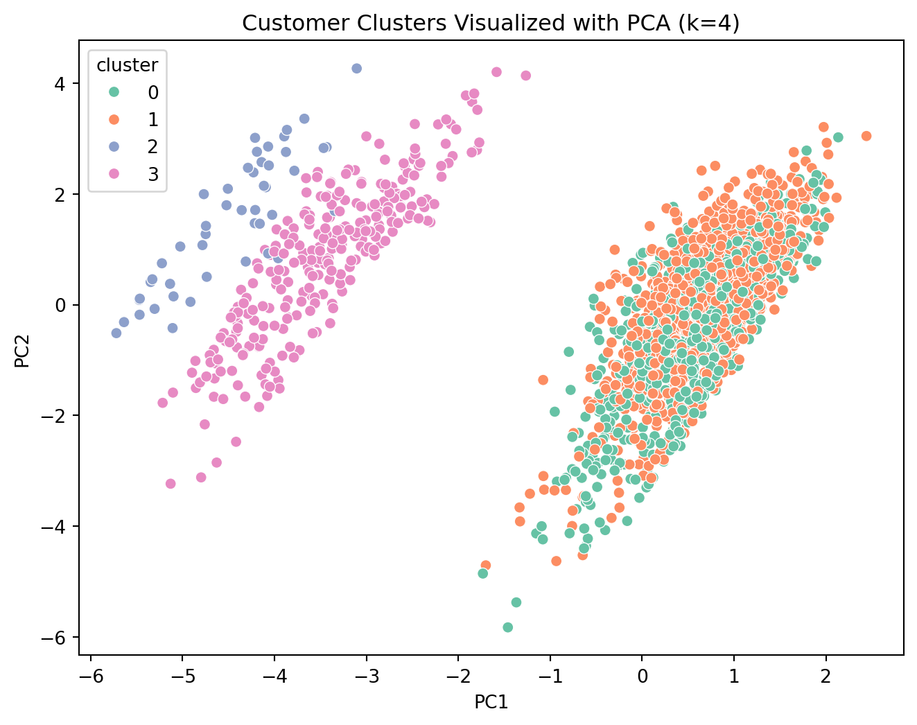
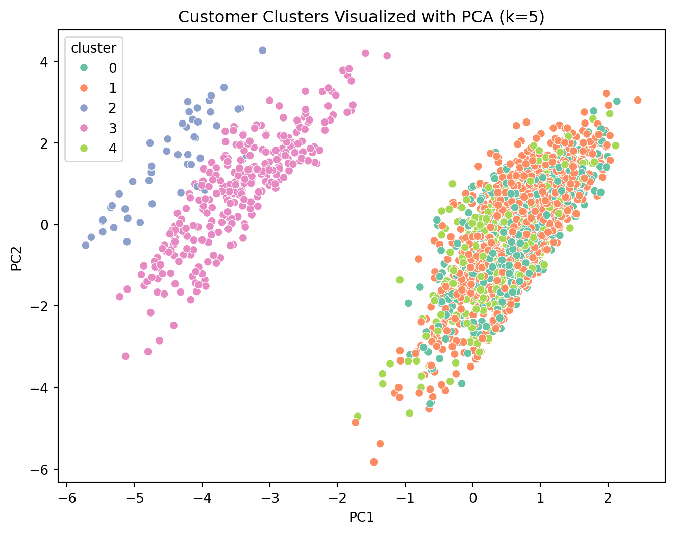
1. **Iterative Clustering**: Run K-Means for *k* from 2 to 5.
2. **Dimensionality Reduction**: Use PCA (Principal Component Analysis) to visualize high-dimensional clusters in 2D.
3. **Evaluation Metrics**: To rigorously assess cluster quality, we analyze the evolution of three distinct metrics as *k* varies:
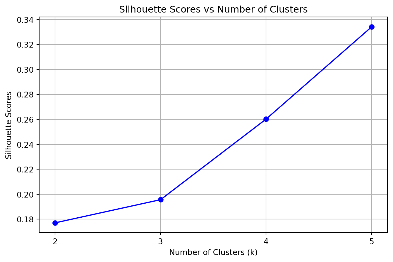
- **Silhouette Score**: Measures the mean distance between a sample and all other points in the same cluster ($a$) versus the mean distance to points in the nearest neighboring cluster ($b$). The score is given by $(b - a) / \max(a, b)$.
- *Evolution*: We look for a peak. A decrease as *k* increases suggests that clusters are becoming less distinct or that natural clusters are being artificially split.
- **Davies-Bouldin Index**: Represents the average similarity between each cluster and its most similar one, where similarity is the ratio of within-cluster scatter to between-cluster separation.
- *Evolution*: We look for a minimum. A rising trend indicates that new clusters are overlapping more or becoming less compact relative to their separation.
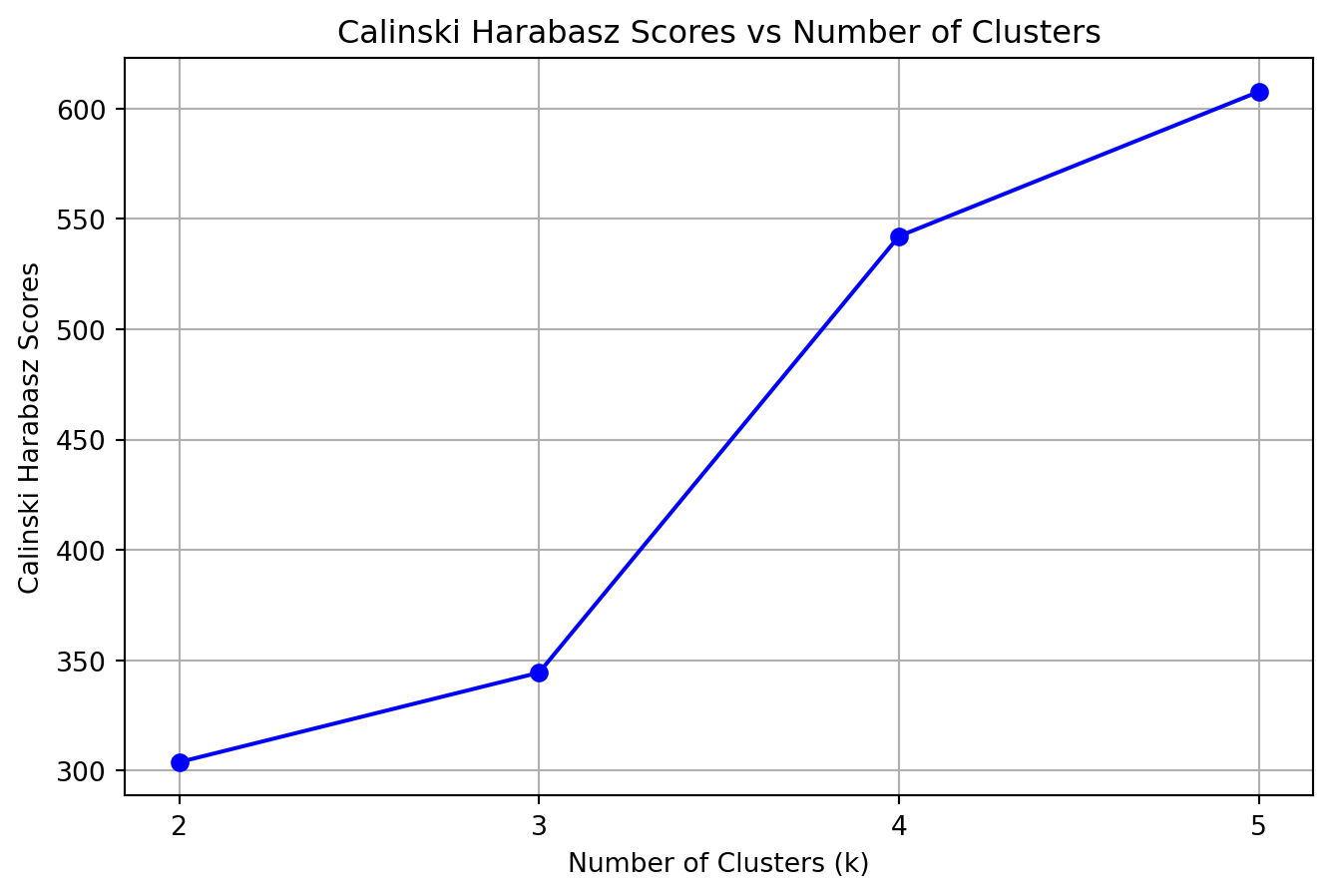
- **Calinski-Harabasz Score**: Also known as the Variance Ratio Criterion, it is the ratio of the sum of between-clusters dispersion and of inter-cluster dispersion for all clusters.
- *Evolution*: We look for a peak. A drop implies that the gain in definition from adding another cluster does not justify the increased complexity (variance).
```{python}
#| code-summary: "Click to see Clustering Functions"
def perform_kmeans_clustering(X_scaled, k_values):
    """
    Execute kmeans clustering algorithm and log the results.
    """
    silhouette_scores = []
    dbi_scores = []
    ch_scores = []
    cluster_data = pd.DataFrame()

    for k in k_values:
        # Perform KMeans clustering
        kmeans = KMeans(n_clusters=k, random_state=42)

        # PCA transformation for viz
        pca = PCA(n_components=2)
        pca_data = pca.fit_transform(X_scaled)
        clusters = kmeans.fit_predict(X_scaled) # Fitting on scaled data, not PCA for accuracy

        # Create a DataFrame for visualization and export
        pca_df = pd.DataFrame(pca_data, columns=['PC1', 'PC2'])
        pca_df['cluster'] = clusters
        pca_df['k'] = k

        # Plot the PCA-transformed data with clusters
        plt.figure(figsize=(8, 6))
        sns.scatterplot(data=pca_df, x='PC1', y='PC2', hue='cluster', palette='Set2')
        plt.title(f"Customer Clusters Visualized with PCA (k={k})")
        plt.show()

        # Calculate scores
        silhouette_scores.append(silhouette_score(X_scaled, clusters))
        dbi_scores.append(davies_bouldin_score(X_scaled, clusters))
        ch_scores.append(calinski_harabasz_score(X_scaled, clusters))

        # Append the current cluster data to the overall DataFrame
        if cluster_data.empty:
            cluster_data = pca_df
        else:
            cluster_data = pd.concat([cluster_data, pca_df], ignore_index=True)

    score_dict = {
        'Silhouette Scores': silhouette_scores,
        'Davies Bouldin scores':dbi_scores,
        'Calinski Harabasz Scores':ch_scores
    }

    return score_dict, cluster_data

def export_model_data(cluster_data, filename):
    cluster_data.to_csv(filename, index=False)
    print(f"Model data exported successfully to {filename}")
```
### Hyperparameter Tuning (Finding optimal k)
We test *k* values from 2 to 6 to find the "elbow" or best performing configuration.
```{python}
k_values = list(range(2, 6))
scoreset, cluster_data = perform_kmeans_clustering(X_scaled, k_values)
# export_model_data(cluster_data, "kmeans_clusters.csv")
```
### Performance Evaluation
We analyse the change in metrics as *k* increases.
```{python}
# Plotting scores
for metric_name, scores in scoreset.items():
    plt.figure(figsize=(8,5))
    plt.plot(k_values, scores, marker='o', linestyle='-', color='blue')
    plt.xticks(k_values)
    plt.xlabel("Number of Clusters (k)")
    plt.ylabel(metric_name)
    plt.title(f"{metric_name} vs Number of Clusters")
    plt.grid(True)
    plt.show()

# Save scores
score_df = pd.DataFrame(scoreset, index=k_values)
# score_df.to_csv("scores.csv", index=True, index_label='k_value')
```
## Selection of Best K
Based on the evaluation metrics:
- **Silhouette Score**: Highest at **k=2**.
- **Davies-Bouldin Score**: Lowest at **k=2**.
- **Calinski-Harabasz Score**: Highest at **k=2**.
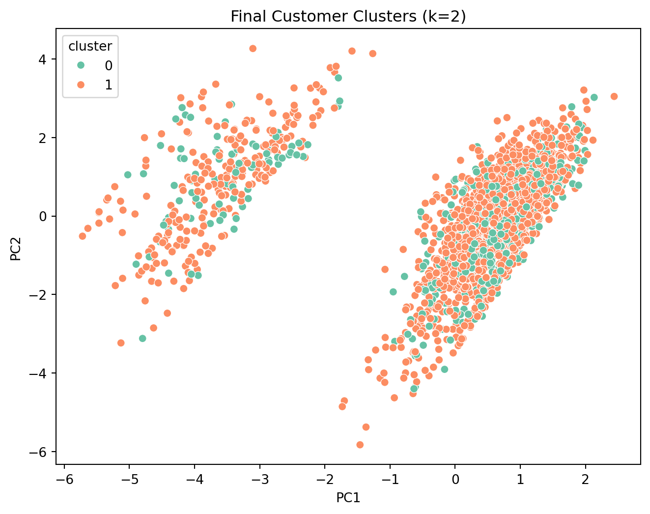
**Conclusion**: We proceed with **k=2** as the optimal number of clusters.
# 8. Basic Inferences (K=2)
We now finalize the model with 2 clusters and analyze the characteristics of each customer segment.
```{python}
# Final Model Execution
kmeans = KMeans(n_clusters=2, random_state=42)
clusters = kmeans.fit_predict(X_scaled)

# Add back to original dataframes
customer_df['cluster'] = clusters
customer_df_original['cluster'] = clusters

# PCA for final visualization
pca = PCA(n_components=2)
pca_data = pca.fit_transform(X_scaled)
pca_df = pd.DataFrame(pca_data, columns=['PC1', 'PC2'])
pca_df['cluster'] = clusters

plt.figure(figsize=(8,6))
sns.scatterplot(data=pca_df, x='PC1', y='PC2', hue='cluster', palette='Set2')
plt.title("Final Customer Clusters (k=2)")
plt.show()
```
### Cluster Profiling
We examine the profile of the two clusters.
```{python}
print("Cluster Counts:")
print(customer_df_original['cluster'].value_counts())
```
**Numeric Feature Summary**
```{python}
numeric_cols = ['avg_order_total', 'total_spent', 'num_orders', 'avg_delay']
summary = customer_df_original.groupby('cluster')[numeric_cols].mean()
print(summary)
```
**Categorical Feature Summary**
```{python}
categorical_cols = ['most_used_payment', 'most_delivery_status']

for col in categorical_cols:
    print(f"Distribution of {col} by cluster:")
    print(customer_df_original.groupby('cluster')[col].value_counts(normalize=True).rename("percentage") * 100)
    print("\n")
```
### Final Interpretation
Based on the profiles, we can label the segments:
- **Cluster 0**: "On-Time High-Value" - High spending, frequent orders, reliable delivery.
- **Cluster 1**: "Delay-Affected Low-Value" - Low spending, infrequent orders, frequent delays.
```{python}
# Mapping cluster names
label_map = {
    0: "On-Time High-Value Customers",
    1: "Delay-Affected Low-Value Customers"
}

customer_df_original['cluster'] = customer_df_original['cluster'].map(label_map)
pca_df['cluster'] = pca_df['cluster'].map(label_map)

# Save result
# customer_df_original.to_csv('results.csv', index=False)

# Final Visual
plt.figure(figsize=(10,6))
sns.scatterplot(data=pca_df, x='PC1', y='PC2', hue='cluster', palette='Set2')
plt.title("Customer Segments")
plt.show()
```
### Conclusion
The analysis reveals that delivery performance is a critical differentiator. High-value customers consistently experience on-time deliveries, while the lower-value segment is plagued by delays. This suggests a potential correlation between service quality and customer value, or perhaps operational issues specifically affecting a subset of orders.